Contents
It is now time for one of the most important topics of theoretical physics. We will learn about the principle of stationary action and how it is used to derive the Euler-Lagrange equation. Pay close attention to the logic of this section, as this approach goes well beyond classical mechanics. This principle gives us a general approach of obtaining the equations of motion of a theory. At the end of this section, we will gain a deeper glimpse of how this principle, as well as the entirety of the Lagrangian formalism, appears in more advanced theories. $\require{physics}$
2.2.1 — The action
The mathematical object in focus for this section is the action $S$. The action is a functional, which means that it takes in a function as its input and spits out a scalar (number) as its output.$^1$ The function which the action takes as its input is the path of the particle, denoted as $q(t)$ (this is just a generalized coordinate with time as a parameter). Hence, we denote the action as $S[q(t)]$, illustrating that it is a functional of the path of a particle.
\begin{equation}\label{eqn:actiondefinition}
S[q(t)] = \int_{t_i}^{t_f} L(q(t), \dot q(t), t) dt
\end{equation}
In other words, the action is the integral of the Lagrangian with respect to time for a certain path $q(t)$ starting from an initial time $t_i$ up to a final time $t_f$. This means that if we pick a specific path for our particle, and we plug it into our action, then we simply get back a number. However, the action will give us a different number if we had picked a different path for the particle.
Yet, out of all the possible paths that a particle could hypothetically take between fixed boundary conditions (the initial and final locations and times), in reality the particle only ends up taking a single path. This true path is the one that minimizes the action. When a path minimizes the action, it means that if we were to apply any small perturbation to the path, while keeping the boundary conditions fixed, then the action will spit out a number that is higher compared to the original path. So the true path that the particle takes is the one whose neighbouring paths (with the same initial and final points) all cause the action to output a larger number compared to the true path. This is known as the Principle of Least Action or Hamilton’s Principle.
It is important to note that the name The Principle of Least Action is actually a misnomer, because it implies that the true path of a particle is the one that always minimizes the action, which is not true in some cases. Sometimes the true path of the particle causes the action to be a maximum (encountered in relativistic theories) or even a saddle point.$^2$ Hence, a more appropriate name is The Principle of Stationary Action, as the term stationary includes minima, maxima, and saddle points all alike. However, in classical mechanics the action can never be maximized. This is because the Lagrangian in classical mechanics takes the form $L=T-U$, and by ignoring relativistic effects, we can make the kinetic energy $T$ of a particle as large as we like (just give the particle a strong kick in its initial condition to give it an arbitrarily large velocity). This will cause the integrand of the action in eq.\eqref{eqn:actiondefinition} to be arbitrarily large. If the action can be made arbitrarily large, then it has no maximum. This logic does not apply beyond classical mechanics, because the definition of the Lagrangian may differ from $L=T-U$.
$^1$ Recall that a regular old function is an object that takes a number as its input and spits back out a number as its output. A generalization of this is the concept of a functional, which takes a whole function as its input and spits out a number as its output.
$^2$ Recall from multivariable calculus that a saddle point is a point along a surface that is neither a maximum or a minimum. It is a point where the surface is a minimum along one direction and a maximum along another direction.
2.2.2 — The principle of stationary action
For the sake of clarity, we will restate the principle of stationary action in a more rigorous form.
\begin{equation}
\delta S[q(t)] = 0
\end{equation}
$\forall \ \delta q(t)$ (for all variations of the path $q$) such that $\delta q(t_i) = \delta q(t_f) = 0$ (fixed boundary conditions).
This requires us to use the machinery of calculus of variations. The symbol $\delta$ means variation (think of a variation as a small change in a function or functional). The expression $\delta S = 0$ is a functional equation, stating that the variation of the action is zero (this shares an analogy with single variable calculus, when the first derivative of a function is zero at a minimum or maximum). The statement $\forall \ \delta q(t)$ means for all variations of the path $q(t)$. Hence, given a set of initial $q(t_i)$ and final $q(t_f)$ conditions, the true path of the particle $q(t)$ is the solution to $\delta S = 0$ for all variations of the path $\delta q(t)$. Lastly, since the boundary conditions are fixed, the variations at the boundaries must vanish $\delta q(t_i) = \delta q(t_f) = 0$. Sometimes this principle is written as $\frac{\delta S}{\delta q} = 0$ to denote that the functional derivative of $S$ vanishes.
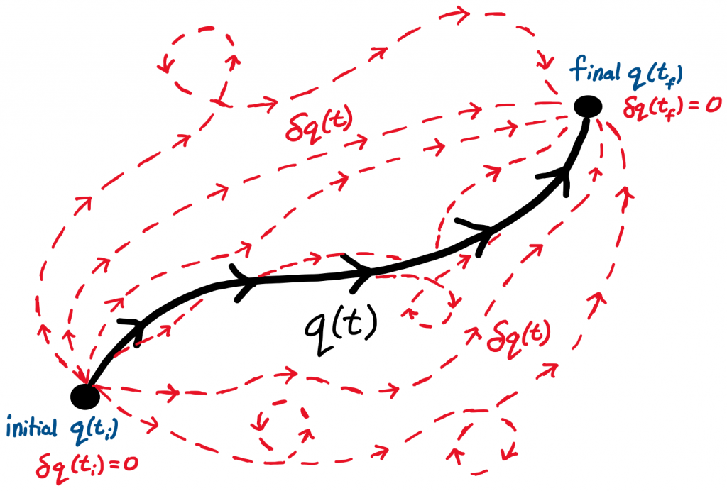
Figure 1. Possible paths for a particle.
Classically, a particle only has one true path that it follows between two points (illustrated in black). However, there are an infinite amount of surrounding paths with the same initial and final destinations that the particle could have taken instead (illustrated in red). Among all the red paths, the true path is the one that causes the action to be stationary, thus obeying the laws of physics.
Before we derive the Euler-Lagrange equation using this action principle, the question jumps straight at us: why does this work? Why do the laws of physics choose a path that causes the action to be stationary? Unfortunately, there is no way to answer this why question within the framework of classical mechanics. For now, take it as an exotic method or definition by which we derive our equations of motion from first principles. However, there is deep physics to be found beneath all of this, and the answer awaits us in the realm of quantum mechanics. But we’re not going to ditch this question just yet. Following our derivation of the Euler-Lagrange equation, we will learn what quantum physics has to teach us about why the principle of least action works!
2.2.3 — Deriving the Euler-Lagrange equation
It is now time to derive the Euler-Lagrange equation for a single classical particle with one degree of freedom. We note the path of the particle as $q(t)$, with a fixed initial point $q(t_i)$ and final point $q(t_f)$. The Lagrangian $L(q(t), \dot q(t), t)$ is a function of the generalized coordinate $q(t)$, generalized velocity $\dot q(t)$, and possibly time $t$. The action is
\begin{equation}
S = \int_{t_i}^{t_f} L(q, \dot q, t) dt
\end{equation}
Let us introduce a small variation $\delta q(t)$ to the path $q(t)$. We will denote this as
\begin{equation}\label{eqn:pathvariation}
q(t) \rightarrow q(t) + \delta q(t)
\end{equation}
This is what will happen: when we introduce a variation to the path, then this will indirectly introduce a variation to the generalized velocity, a variation to the Lagrangian, as well as a variation to the action.
\begin{equation}
\dot q \rightarrow \dot q + \delta \dot q
\end{equation}
\begin{equation}
L \rightarrow L + \delta L
\end{equation}
\begin{equation}
S \rightarrow S + \delta S
\end{equation}
Our goal is to elucidate what these variations $\delta L$ and $\delta S$ actually look like. Once we accomplish this, we can simply set the variation of the action to zero $\delta S = 0$, and by our action principle, this should give rise to our equation of motion!
Let’s first begin with the variation to the generalized velocity. This one is actually simpler than it looks, but throughout this derivation keep track of all the dots on top of the $\dot q$’s (sometimes it’s hard to see the dots on a webpage). Recall that the notation $\dot q$ means $\frac{dq}{dt}$. So the variation $\delta \dot q$ means $\delta \frac{dq}{dt}$. It turns out that the variation operator $\delta$ commutes with the regular derivative operator $\frac{d}{dt}$ (it also commutes with integrals). Hence, we have
\begin{equation}\label{eqn:velocityvariation}
\delta \dot q = \frac{d}{dt} \delta q
\end{equation}
The variation of the Lagrangian is a bit more involved, since it is a function of $q(t)$ and $\dot q(t)$, both of which have variations themselves. We know that $q \rightarrow q + \delta q$ and $\dot q \rightarrow \dot q + \delta \dot q$, so the Lagrangian transforms as
\begin{equation}
L(q, \dot q, t) \rightarrow L(q+\delta q, \dot q + \delta \dot q, t)
\end{equation}
The transformed Lagrangian $L(q+\delta q, \dot q + \delta \dot q, t)$ must look like $L(q, \dot q, t) + \delta L$. This approximation arises from a first-order Taylor expansion with respect to the variation $\delta q$:
\begin{equation}
L(q+\delta q, \dot q + \delta \dot q, t) = L(q, \dot q, t) + \pdv{L}{q} \delta q + \pdv{L}{\dot q} \delta \dot q + \mathcal{O}(\delta q^2)
\end{equation}
Since we are only keeping terms up to first order in $\delta q$, we can neglect the higher-order terms $\mathcal{O}(\delta q ^2)$. In other words, we are taking the variations (or perturbations) in the path $q(t)$ to be very small. So we have
\begin{equation}\label{eqn:taylorexpandlagrangian}
L(q, \dot q, t) \rightarrow L(q, \dot q, t) + \underset{= \ \delta L}{\bbox[5px, border: 1px dashed #800020]{\pdv{L}{q}\delta q + \pdv{L}{\dot q}\delta \dot q}}
\end{equation}
The variation of the Lagrangian to first order is therefore $\delta L = \pdv{L}{q}\delta q + \pdv{L}{\dot q} \delta \dot q$.
So far so good, but what happens to the action? Similar to the Lagrangian, we know the action transforms as
\begin{equation}
S[q] \rightarrow S[q+\delta q] = S[q] + \delta S[q]
\end{equation}
The transformed action $S[q+\delta q]$ can simply be expressed as the transformed Lagrangian $L(q+\delta q, \dot q + \delta \dot q, t)$.
\begin{equation}
S[q+\delta q] = \int_{t_i}^{t_f} L(q+\delta q, \dot q + \delta \dot q, t) dt
\end{equation}
But we know the form of the transformed Lagrangian from eq.$\eqref{eqn:taylorexpandlagrangian}$, so
\begin{equation}
S[q+\delta q] = \int_{t_i}^{t_f} \Big( L + \pdv{L}{q}\delta q + \pdv{L}{\dot q} \delta \dot q \Big) dt
\end{equation}
Let’s separate the first term in the integrand from the rest.
\begin{equation}
S[q+\delta q] = \underset{= \ S}{\bbox[5px, border: 1px dashed #800020]{\int_{t_i}^{t_f} L dt}} + \underset{= \ \delta S}{\bbox[5px, border: 1px dashed #800020]{\int_{t_i}^{t_f} \Big( \pdv{L}{q} \delta q + \pdv{L}{\dot q} \delta \dot q \Big) dt}}
\end{equation}
We got what we were looking for, the second term is the variation of the action $\delta S$. By the principle of stationary action, all we need to do is set $\delta S = 0$ and see what pops out. Before we do that, however, we should manipulate the integral to make it a bit more manageable.
\begin{equation}
\delta S = \int_{t_i}^{t_f} \Big( \pdv{L}{q}\delta q + \pdv{L}{\dot q} \delta \dot q \Big) dt
\end{equation}
First, we’ll use our result from eq.$\eqref{eqn:velocityvariation}$ where we found that $\delta \dot q = \frac{d}{dt}\delta q$.
\begin{equation}
\delta S = \int_{t_i}^{t_f} \Big( \pdv{L}{q}\delta q + \pdv{L}{\dot q} \frac{d}{dt}\delta q \Big) dt
\end{equation}
Now we will perform integration by parts on the second term in the integrand.
\begin{equation}
\int_{t_i}^{t_f} \pdv{L}{\dot q} \Big(\frac{d}{dt} \delta q \Big) dt = \int_{t_i}^{t_f} \frac{d}{dt} \Big( \pdv{L}{\dot q} \delta q \Big)dt- \int_{t_i}^{t_f} \Big( \frac{d}{dt} \pdv{L}{\dot q} \Big) \delta q dt
\end{equation}
By the fundamental theorem of calculus, the first term (integral of a full derivative) of the above equation simply becomes an evaluation at the boundaries.
\begin{equation}
\int_{t_i}^{t_f} \pdv{L}{\dot q} \Big(\frac{d}{dt} \delta q \Big) dt = \pdv{L}{\dot q} \delta q \Bigg|_{t=t_i}^{t=t_f}-\int_{t_i}^{t_f}\Big(\frac{d}{dt}\pdv{L}{\dot q} \Big) \delta q dt
\end{equation}
At first sign it seems like the integration by parts technique didn’t make our life easier. But looking at the first term of the above equation, it evaluates $\pdv{L}{\dot q}\delta q$ at $t=t_i$ and $t=t_f$:
\begin{equation}
\pdv{L}{\dot q}\delta q \Bigg|_{t=t_i}^{t=t_f} = \pdv{L(t_f)}{\dot q} \underset{= \ 0}{\bbox[5px, border: 1px dashed #800020]{\delta q(t_f)}}- \pdv{L(t_i)}{\dot q} \underset{= \ 0}{\bbox[5px, border: 1px dashed #800020]{\delta q(t_i)}} = 0
\end{equation}
The variations of the path at the boundaries vanish because, when we began this journey, we asserted that the boundaries remain fixed. This is the entire reason why we bothered to do integration by parts.
Returning back to our action and using this result, we have
\begin{equation}
\delta S = \int_{t_i}^{t_f} \Big( \pdv{L}{q} \delta q- \Big(\frac{d}{dt} \pdv{L}{\dot q}\Big) \delta q \Big) dt
\end{equation}
The integration by parts technique effectively allowed us to switch the $\frac{d}{dt}$ operator from $\delta q$ over to the $\pdv{L}{\dot q}$ term. Now both terms in the integrand have a common $\delta q$ term, so we can factor it out.
\begin{equation}
\delta S = \int_{t_i}^{t_f} \Big(\pdv{L}{q}-\frac{d}{dt} \pdv{L}{\dot q} \Big) \delta q dt
\end{equation}
Now we are in a position to set $\delta S = 0$ by the principle of stationary action and obtain our equation of motion.
\begin{equation}
\delta S = 0 \Longleftrightarrow \int_{t_i}^{t_f}\Big(\pdv{L}{q}-\frac{d}{dt}\pdv{L}{\dot q}\Big)\delta q dt = 0, \ \forall \ \delta q
\end{equation}
Note that throughout this discussion, we didn’t specify anything about $\delta q$, other than it being a small perturbation. So the integral must vanish for all $\delta q$. By a fundamental theorem in the calculus of variations, this is only possible if the term inside the brackets vanishes.$^3$
Hence,
\begin{equation}
\delta S = 0 \Longleftrightarrow \pdv{L}{q}- \frac{d}{dt} \pdv{L}{\dot q} = 0
\end{equation}
Rearranging gives the Euler-Lagrange equation.
\pdv{L}{q} = \frac{d}{dt} \pdv{L}{\dot q}
\end{equation}
The true path of the particle $q(t)$ is the one that satisfies the Euler-Lagrange equation, a second-order partial differential equation. The principle of stationary action gave us the fundamental equation of motion in Lagrangian mechanics.
$^3$ A fundamental theorem in the calculus of variations says that, if we have an equation of the form $\int_{t_i}^{t_f} f(q)\delta q dt = 0$ for a general function $f(q)$ and any variation $\delta q$, then it implies that $f(q)=0$.
Exercises
2.3 — *Explicit minimization of the action. In this problem, we are going to explicitly find the true path of a particle by directly minimizing the action. Consider a particle of mass $m$ moving along the $y$-axis. The particle is near the Earth’s surface and experiences a gravitational potential of $U(y)=-mgy$, where $y$ is the height of the particle above the ground and $g$ is a constant. Assume that the path of the particle can be written as a function of time as $y(t)=At^2+Bt+C$, where $A$, $B$, and $C$ are constants. At $t=0$ the particle starts at $y(0)=0$, and at $t=T$ the particle ends at $y(T) = h$. By directly minimizing the action, find the value of the constants $A$, $B$, and $C$.
2.4 — **Higher-order Euler-Lagrange equations. For the sake of curiosity, assume that a Lagrangian is a function of not only the coordinate $q$ and its first-order derivative $\dot q$, but also its second-order derivative $\ddot q$, so that $L=L(q, \dot q, \ddot q, t)$. Assume that the new boundary conditions are such that the variations of the coordinate at the boundaries vanish $\delta q(t_i)=\delta q(t_f)=0$, and the variations of the velocity at the boundaries vanish as well $\delta \dot q(t_i)=\delta \dot q(t_f) = 0$. In a similar fashion to how we derived the Euler-Lagrange equation, use the principle of stationary action to prove that the higher-order Euler-Lagrange equation that corresponds to this new case is
\begin{equation}
\pdv{L}{q} = \frac{d}{dt} \pdv{L}{\dot q}- \frac{d^2}{dt^2} \pdv{L}{\ddot q}
\end{equation}
For those want to go all the way, assume that a Lagrangian is now a function of $n$ derivatives of the coordinate $q$, so that $L=L(q, \frac{dq}{dt}, \frac{d^2q}{dt^2}, \frac{d^3q}{dt^3},\ldots, \frac{d^nq}{dt^n}, t)$. Assume that the variations of the coordinate at the boundaries vanish, and that the variations of all the derivatives of the coordinate (up to the $(n-1)^\text{th}$ derivative) also vanish. Using the principle of stationary action, prove that the corresponding Euler-Lagrange equation is
\begin{equation}
\pdv{L}{q}+\sum_{k=1}^{n}(-1)^k\frac{d^k}{dt^k}\pdv{L}{q^{(k)}}=0
\end{equation}
where the notation $q^{(k)} \equiv \frac{d^kq}{dt^k}$ simplifies writing all of the derivatives of $q$. Don’t worry about all of these higher-order Euler-Lagrange equations, as we’ll never see them in practice. The purpose of this problem is to exercise our action-principle skills.