Before we introduce the Lagrangian, we need to introduce the notion of degrees of freedom and generalized coordinates. $\require{physics}$

2.1.1 — Degrees of freedom

Imagine a particle moving in three spatial dimensions. We use the position vector $\vb{r}=(x,y,z)$ to specify its position in Cartesian coordinates. Of course, we could have equally well used another coordinate system, such as cylindrical coordinates $\vb{r} = (\rho, \phi, z)$ or spherical coordinates $\vb{r}=(r, \theta, \phi)$. Notice that these three approaches have one thing in common: three independent pieces of information pertaining to the particle’s position. For instance, $\vb{r}=(x,y,z)$ lists how far the particle is along the $x$-, $y$-, and $z$-axes, while $\vb{r}=(r,\theta,\phi)$ lists the particle’s distance $r$ from the origin, the angle $\theta$ between the position vector and the $z$-axis, and the angle $\phi$ between the projection of the position vector (onto the $xy$-plane) and the $x$-axis.

These independent pieces of information are called degrees of freedom. More precisely, a degree of freedom is a direction in which a particle can move along independently of other directions and other particles. To completely specify the position of a particle, we need to list all of its degrees of freedom. In the above example, we needed three degrees of freedom because the particle was moving freely in three spatial dimensions. The label of the degrees of freedom depends on the chosen coordinate system, but the number of degrees of freedom must be the same regardless of what coordinate system we use. For instance, if a particle is moving freely in two spatial dimensions, we could label the degrees of freedom as $\{x,y\}$ in Cartesian coordinates or as $\{r, \phi\}$ in polar coordinates. In both cases, however, there are only two degrees of freedom.

What if we had two particles in three dimensions? Then there are six degrees of freedom, three from the first particle $\vb{r}_1=(x_1,y_1,z_1)$ and three from the second particles $\vb{r}_2=(x_2,y_2,z_2)$. In general, if there are $N$ particles moving freely in $D$ spatial dimensions, there are $N\times D$ degrees of freedom in total.

In this context, the degrees of freedom are associated with the physical configuration of the system (describing the locations of all the particles). However, this is not enough to completely describe the motion of the entire system. In order to do this, we also need to specify the velocity of each particle in addition to the physical configuration of the system. There is a neat fact that each degree of freedom is uniquely paired with its own velocity. For instance, a particle moving freely in three spatial dimensions has three degrees of freedom $\{x, y, z \}$, with each degree of freedom being associated with its own velocity $\{v_x, v_y, v_z \}$. To completely describe the motion of a system, we need to know all the degrees of freedom as well as their velocities.

Notice that degrees of freedom are independent parameters. For example, for two particles moving freely in two dimensions, the degrees of freedom are $\{x_1, y_1, x_2, y_2 \}$ (the numerical subscripts refer to particles 1 and 2). Specifying the $x$-position of particle 2 ($x_2$) gives no information regarding the degrees of freedom associated with particle 1 $\{x_1,y_1 \}$, nor the $y$-position of particle 2 ($y_2$). The same holds true if were to specify any of the other degrees of freedom, and hence, degrees of freedom are independent parameters. It also turns out that the velocity associated with each degree of freedom is also independent of all the other velocities as well as all the degrees of freedom. For instance, specifying the $y$-component of velocity for particle 1 ($v_{y1}$) gives no information regarding any other component of velocity nor any degree of freedom.

Sometimes, however, the number of degrees of freedom are less than what we expect for $N$ particles in $D$ spatial dimensions. This can occur if our system exhibits a constraint. A constraint is any restriction of the motion of any particle in the system.

For example, how many degrees of freedom are there for a particle at the end of a pendulum of length $\ell$ that is swinging to the left and right while hanging from the ceiling? Although we can think of the particle as existing in three dimensions, it is not moving freely in three dimensions. Its motion is constrained to be within a two-dimensional plane created by the swing of the pendulum. Furthermore, due to the nature of the pendulum, the particle is always a distance $\ell$ away from the point where the pendulum is attached to the ceiling. If we think of the point of attachment to the ceiling as the origin, with the $x$-axis serving as the vertical and the $y$-axis along the ceiling, then the particle’s position is given by the coordinates $(\ell, \phi)$ in polar coordinates. Since the length of the pendulum $\ell$ is a constant while $\phi$ can change, the particle’s position is completely specified if we know $\phi$, which is the angle between the pendulum and the vertical.

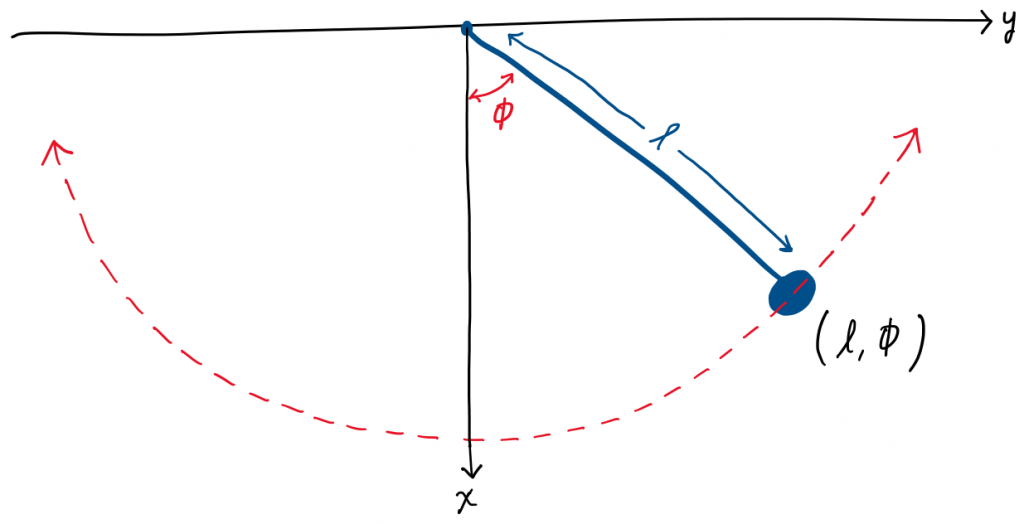
Figure 1. Swinging pendulum.

A pendulum of fixed length swinging in a two-dimensional plane has only one degree of freedom, which can be expressed as the angle $\phi$ in polar coordinates.

Hence, there is only one degree of freedom. This degree of freedom $\phi$ has a velocity $\dot \phi$, which is the angular velocity of the particle (the speed at which the particle moves along the circular arc created by the swinging pendulum). The motion of the system is completely specified by the pair of parameters $\{\phi, \dot \phi \}$.

$^1$ You may rightfully wonder why our discussion of degrees of freedom does not include velocities. For freely moving particles, velocities are indeed independent parameters that are needed to specify the motion of a system, but this awfully sounds very similar to the definition of a degree freedom. However, we are making a distinction that degrees of freedom are tied to the configuration of a system (the locations of all the particles, not their velocities). When we discuss Hamiltonian mechanics, this distinction will be more clear. For those who are curious, the number of degrees of freedom for a system is the dimensionality of its configuration space. For $N$ particles moving freely in $D$ spatial dimensions, the entire configuration of this system is a point located on a ($N \times D$)-dimensional manifold (its configuration space). If we also take into account their velocities (or more precisely, their momenta), then we start to discuss a similar concept known as phase space. Since each degree of freedom is tied to a unique velocity, this system of free particles can be described by a ($2\times N\times D$)-dimensional phase space.

2.1.2 — Generalized coordinates

Wouldn’t it be nice if we could focus on the intuition behind classical mechanics without worrying which coordinate system we are using? This is where the idea of generalized coordinates comes in.

Instead of worrying whether to use $\{x,y,z\}$, $\{\rho, \phi, z\}$, $\{r, \theta, \phi \}$, or any of the countless coordinate systems we can conjure up, we instead use a generalized coordinate system denoted as $\{q\}$. The notation $\{q\}$ represents a set (the curly braces) of generalized coordinates $q$ that we are referring to. Each $q$ represents a degree of freedom, much like how each $x$, $y$, and $z$ represented a degree of freedom in the previous section.

Each generalized coordinate $q$ is associated with its own generalized velocity $\dot q$ (pay attention to the dot over the $\dot q$, which is a bit hard to see on this webpage).$^2$

\begin{equation}\label{eqn:genvelocity}
\dot q \equiv \frac{d q}{dt}
\end{equation}

There are many ways in which this notation can be used. We will go over a couple of ways below.

• One particle moving freely in three spatial dimensions.
  • $\{q_i\} \equiv \{q_1, q_2, q_3 \}$ lists three degrees of freedom equivalent to $\{x,y,z\}$ in Cartesian coordinates, or $\{\rho, \phi, z\}$ in cylindrical coordinates, or $\{r, \theta, \phi \}$ in spherical coordinates.
  • $\{ \dot q_i\} \equiv \{\dot q_1, \dot q_2, \dot q_3 \}$ lists the three velocities equivalent to $\{\dot x, \dot y, \dot z \}$ in Cartesian coordinates, or $\{\dot \rho, \dot \phi, \dot z\}$ in cylindrical coordinates, or $\{\dot r, \dot \theta, \dot \phi \}$ in spherical coordinates.
• Two particles moving freely in two spatial dimensions.
  • $\{q_i\} \equiv \{q_1, q_2, q_3, q_4 \}$ lists four degrees of freedom equivalent to $\{x_1, y_1, x_2, y_2 \}$ in Cartesian coordinates or $\{r_1, \phi_1, r_2, \phi_2 \}$ in polar coordinates.
  • $\{\vb{q}\} \equiv \{\vb{q}_1, \vb{q}_2 \}$ also lists four degrees of freedom, but shortens the notation by using $\vb{q}_1 \equiv \vb{r}_1 = (x_1, y_1)$ and $\vb{q}_2 \equiv \vb{r}_2 = (x_2, y_2)$ as the position vectors of particles 1 and 2, respectively.

We will stick with the notation $\{q_i\}$ as it is more clear. To make life easier, we’ll write it as $\{q\}$ (without the subscript). Remember that $\{q\}$ denotes the set of all degrees of freedom for a system. Likewise, $\{\dot q \}$ denotes the set of all the velocities corresponding to the degrees of freedom for a system.

How do we write down our expressions for the kinetic energy $T$ and potential energy $U$ of a system using these generalized coordinates? Recall that the kinetic energy of a system is a function of the velocities of all the particles in a system. If there are $N$ particles of mass $m$ moving freely in three spatial dimensions, then the total kinetic energy can be written as

\begin{equation}\label{eqn:kineticenergygeneral}
T \equiv T(\{\dot q \}) = \sum_{i=1}^{3N}\frac{1}{2}m(\dot q_i)^2
\end{equation}

The notation $T(\{\dot q_i\})$ means that $T$ is a function of the set of the generalized velocities of all the degrees of freedom (try to reason out why the above sum is taken from $i=1$ to $i=3N$). Likewise, for classical systems whose potential energy is only a function of the positions of all the particles in a system, the potential energy can be written as

\begin{equation}\label{eqn:potentialenergygeneral}
U \equiv U(\{q\})
\end{equation}

This tells us that $U$ is a function of the generalized coordinates of the system. The exact form of $U$ depends on what kind of system we are discussing (e.g., gravitational potential energy, electrostatic potential energy, spring potential energy, etc.). Lastly, if we have an object $F$ that is a function of the generalized coordinates and the generalized velocities of a system, we can write it as

\begin{equation}\label{eqn:functiongeneral}
F \equiv F(\{q\}, \{\dot q\})
\end{equation}

Sometimes we’re lazy and we’ll simply write it as $F(q,\dot q)$, where it is understood that $F$ is a function of the sets of generalized coordinates and velocities.

Now we can expand on the idea of the constraints that we introduced a bit earlier.

Let’s apply this reasoning to our previous pendulum example. If we treat the pendulum as existing within a broader three-dimensional landscape, how can we mathematically express its constraints? The first constraint is that the pendulum is only swinging to the left and right within a plane, and if we imagine orienting the $z$-axis perpendicular to this plane, we can express this constraint as $z=0$. We could have instead used $z=5$ or $z=-100$ by shifting the $z$-axis, but it doesn’t matter, as any equation of that form restricts the movement of the particle to a plane. How about the constraint of the particle being a fixed distance $\ell$ away from the origin? Well, we can think of the particle as only being able to move along a circle of radius $\ell$, and in Cartesian coordinates this would be expressed as $x^2+y^2=\ell^2$. These two equations $z=0$ and $x^2+y^2-\ell^2=0$ represent the two constraints of the system, and they are in fact holonomic constraints. A free particle in three dimensions has three degrees of freedom, but since the pendulum introduces two holonomic constraints, the final number of degrees of freedom reduces to $3-2=1$. This matches our previous conclusion that, in polar coordinates, the single degree of freedom $\phi$ is sufficient to describe the position of the particle.

$^2$ We will use the notation $\equiv$ to mean “equivalent to” or “defined as”. So, in general, when we have $A \equiv B$, it is not a statement that provides any physics insight, but rather a definition or an illustration of how two notations are equivalent.

2.1.3 — The Lagrangian

The goal of Lagrangian mechanics is to focus on an object called the Lagrangian, denoted as $L$, to obtain all the information we need about the dynamics of a system. How we exactly obtain the equations of motion from this curious object is discussed in the next section. Here we simply describe what it is.

Note that we mentioned $L$ may have an explicit dependence on time. This means, depending on the nature of the system, the parameter for time $t$ may explicitly appear in $L$ once we express $T$ and $U$. This usually occurs if there is an external influence on $T$ or $U$ that varies with time.$^4$ However, $L$ always has an implicit dependence on time. An implicit dependence on time means that $L$ still varies with time, even if $t$ does not explicitly appear in the expression for $L$, because the coordinates $q \equiv q(t)$ and velocities $\dot q \equiv \dot q(t)$ themselves directly vary with time.

Example 1. Spring on a cone. Express the Lagrangian for a particle of mass $m$ stuck to move on the surface of a cone. The particle is attached to a spring that is anchored at the origin (the tip of the cone). The spring has a spring constant $k$ and an equilibrium length of $d$. The surface of the cone makes an angle of $\alpha$ with the vertical.

Solution. First, we should choose an appropriate coordinate system for this problem. Any coordinate system would work, but some are more suitable for certain problems than others. In this case, we notice that the opening angle of the cone $\alpha$ plays the same role as the polar angle $\theta$ in spherical coordinates. Hence, the particle lives on a cone defined by the surface $\theta = \alpha$ (this actually expresses a holonomic constraint of our system in mathematical form). In spherical coordinates, the position of this particle is given by $\vb{r}=(r, \alpha, \phi)$. A particle in three spatial dimensions with one constraint has two degrees of freedom. In this case, the two degrees of freedom are $r$ and $\phi$ since they can independently vary from $0 \leq r < \infty$ and $0 \leq \phi \leq 2\pi$, while $\theta = \alpha$ is a constant.

Next, having chosen our coordinate system and determined our degrees of freedom, we should find the kinetic energy. Typically, we start with the expression for $T$ in Cartesian coordinates as

\begin{equation}
T(\dot x, \dot y, \dot z) = \frac{1}{2}m(\dot x^2 + \dot y^2 + \dot z^2)
\end{equation}

and use the appropriate change of variables to spherical coordinates.

\begin{equation}
\begin{alignedat}{1}
&x=r\sin(\alpha)\cos(\phi) \\
&y=r\sin(\alpha)\sin(\phi) \\
&z=r\cos(\alpha)
\end{alignedat}
\end{equation}

Next, we find the velocities $\dot x$, $\dot y$, $\dot z$ by taking the time derivative of the above three equations, and then substitute them into the expression for $T$. After using the chain rule, we should arrive at

\begin{equation}
\begin{alignedat}{1}
&\dot x = \Big(\dot r\cos(\phi)-r\sin(\phi)\dot \phi \Big)\sin(\alpha) \\
&\dot y = \Big(\dot r\sin(\phi)+r\cos(\phi)\dot \phi \Big)\sin(\alpha) \\
&\dot z = \dot r \cos(\alpha)
\end{alignedat}
\end{equation}

Substituting these expressions back into $T$ gives us

\begin{equation}
T(\dot r, \dot \phi) = \frac{1}{2}m\Big(\dot r ^2 + r^2\sin^2(\alpha)\dot \phi^2 \Big)
\end{equation}

We are done with the kinetic energy. Now we move onto the potential energy $U$, which in this system, is the spring energy. If the equilibrium length of the spring is $d$, and the particle’s distance from the origin is $r$, then the spring is displaced a distance of $r-d$ from its equilibrium point. The potential energy is therefore

\begin{equation}
U(r) = \frac{1}{2}k(r-d)^2
\end{equation}

Hence, the Lagrangian of the system is

\begin{equation}
\begin{alignedat}{1}
&L(r, \phi, \dot r) = T – U \\
&L(r, \phi, \dot r) = \frac{1}{2}m\Big(\dot r^2 + r^2\sin^2(\alpha)\dot \phi^2 \Big) – \frac{1}{2}k(r-d)^2
\end{alignedat}
\end{equation}

At this point it may seem mysterious why such an object is so important. It looks like $L=T-U$ is almost identical to the total energy $E=T+U$ of a system, but it has that pesky minus sign instead! The beauty of Lagrangian mechanics will be explored in the next two sections, where we’ll use the Lagrangian to obtain the equations of motion of any system.

$^3$ This expression of the Lagrangian is used in classical mechanics. Once we delve into relativity and quantum field theory, the expression for the Lagrangian becomes more complicated.
$^4$ In the context of electromagnetism, think of someone periodically flipping a switch to alter the magnitude of an external electric field to control the motion of charged particles.

Exercises

2.1 — Degrees of freedom. List the degrees of freedom and corresponding velocities for the following systems by picking an appropriate coordinate system (assume all particles each have mass $m$).

• (a) Cone. N particles stuck to move on the surface of a cone, whose surface makes an angle of $\theta$ with respect to the $z$-axis.
• (b) Wire. Three beads slide along a wire connected to a wire connected to a wall at each end, with the wire having an arbitrary shape with many curves and turns.
• (c) *Coupled pendulums. A particle at the end of a pendulum of length $\ell_1$, attached to the start of another pendulum of length $\ell_2$ whose end has a second particle, with both pendulums swinging in a two-dimensional plane.

2.2 — Lagrangians. Express the Lagrangian of the following systems using the given coordinate systems. Which system(s) have a Lagrangian with an explicit time dependence?

• (a) Spherical and springs. One particle of mass $m$ attached to the origin via a spring with a spring constant $k$ and an equilibrium length of zero.
• (b) Cylindrical and external potentials. Three particles of mass $m$ stuck on the surface of an infinite cylinder of radius $R$, experiencing a potential of $U=-kz$, where $k$ is a positive constant.
• (c) Cartesian and gravity. Two particles of mass $m_1$ and $m_2$ moving freely in three spatial dimensions and interacting via gravity.
• (d) *Polar and a forced rod. One particle of mass $m$ free to slide along an infinite massless rod, whose midpoint is attached at the origin, and which rotates about the origin (within a plane) at an angular velocity that increases linearly with time $\dot \phi = kt$, where $k$ is a constant and $t$ is time.